eea_s42.htm

231001 'HAND' http://farbe.li.tu-berlin.de/eea_s42.htm or http://color.li.tu-berlin.de/eea_s42.htm.

Project title: Colour and colour vision with Ostwald, device, and elementary colours -
Antagonistic colour-vision models TUBJND and TUBLAB, and properties for many applications

Chapter E: Colour Metrics, Differences, and Appearance (2023), Main part eea_s, under work

Titles and links to six different topics (all under work in 2023)
Title of part 4.1: Achromatic colour metric for the surface colour range for adjacent (a) and separated (s) samples
eea_s41 in English or ega_s41 in German.

Title of part 4.2: Achromatic and chromatic colour metric for the surface colour range
eea_s42 in English or ega_s42 in German.

Title of part 4.3: Achromatic colour metric for a wide luminance range between the Low, Standard and High Dynamic Range (LDR, SDR, and HDR)
eea_s43 in English or ega_s43 in German.

Title of part 4.4: Achromatic and chromatic colour metric for a wide luminance range between the Low, Standard and High Dynamic Range (LDR, SDR, and HDR)
eea_s44 in English or ega_s44 in German.

Title of part 4.5: Research results and connections of special CIE and TUB colourimetries
eea_s45 in English or ega_s45 in German.

Title of part 4.6: Research results on the colour appearance attribute colourfullness
eea_s46 in English or ega_s46 in German.

For links to the main chapter E
Colour Metrics, Differences, and Appearance (2023), under work.
Content list of chapter E (links and file names use small letters), see
eea_s in English or ega_s in German.
_________________________

Title of part 4.2: Achromatic and chromatic colour metric for the surface colour range

4.21. Introduction: Definition and wavelength limits of Ostwald-optimal colours.
Richter (2020) has studied the colorimetric properties of the complementary Ostwald-optimal colours, see Fig. 4.21-1.

Figure 4.21-1: Wavelength limits of two complementary Ostwald-optimal colours
For the download of this figure in the VG-PDF format, see eeh91-5a.pdf.

Two complementary Ostwald-optimal colours, for example yellow and blue, consist of a colour half. The two colour halfs are shown by broken lines, for example the two special pairs Yellow-Blue and Red-Cyan. Other two colour halfs are produced by the green lines.

The spectral power distribution of 8 Planck (Pxx) illuminants with colour temperatures between 3000K and 6500K define both the (x, y) chromaticity of the illuminant and the wavelength limits of the pairs Yellow-Blue and Red-Cyan, see Fig. 4.21-2.

Figure 4.21-2: Wavelength limits of two pairs of complementary Ostwald-optimal colours for 8 Planck illuminants Pxx
For the download of this figure in the VG-PDF format, see eeh90-7n.pdf.

Two complementary Ostwald-optimal colours consist of a colour half, for example yellow and blue. The two colour halfs are produced by the broken black lines.

A change of the spectral power distribution from P65 to P30 increase the colour temperature, and changes the chromaticity of the illuminant and the wavelength limits from lamda = 494 nm to 507 nm. There are similar changes for the CIE standard illuminants D65, D50, and A (called A00 here) and 5 other illuminants, see Fig. 4.21-3

Figure 4.21-3: Wavelength limits of two pairs of complementary Ostwald-optimal colours for 8 Daylight illuminants Dxx
For the download of this figure in the VG-PDF format, see eeh91-7n.pdf.

All illuminants between P65 and P30 produce approximately the same tristimulus value ratio between Yellow (Y) and Blue (B). The ratio YYellow : YBlue = 13 : 1 is approximately constant for the eight illuminants.

An explanation seems the following: For the change from P65 to P30 the spectral power increases in the yellow-red area. However the wavelength range decreases. Therefore the tristimulus value of Yellow may be approximately constant. If this is true, then the tristimulus value of Blue is also constant because both mix to white.

The colour temperature of the CIE standard inlluminants D65, D50 and A change in the same range, see the above Fig. 4.21-3

4.22: Constant tristimulus values Yo=o of Ostwald colours (o) for a wide range of chromatic adaptation between 6500K and 3000K.
For the tristimulus values, wavelength limits, chromaticities and chromatic values for the standard illuminant D50, see Fig. 4.22-1.

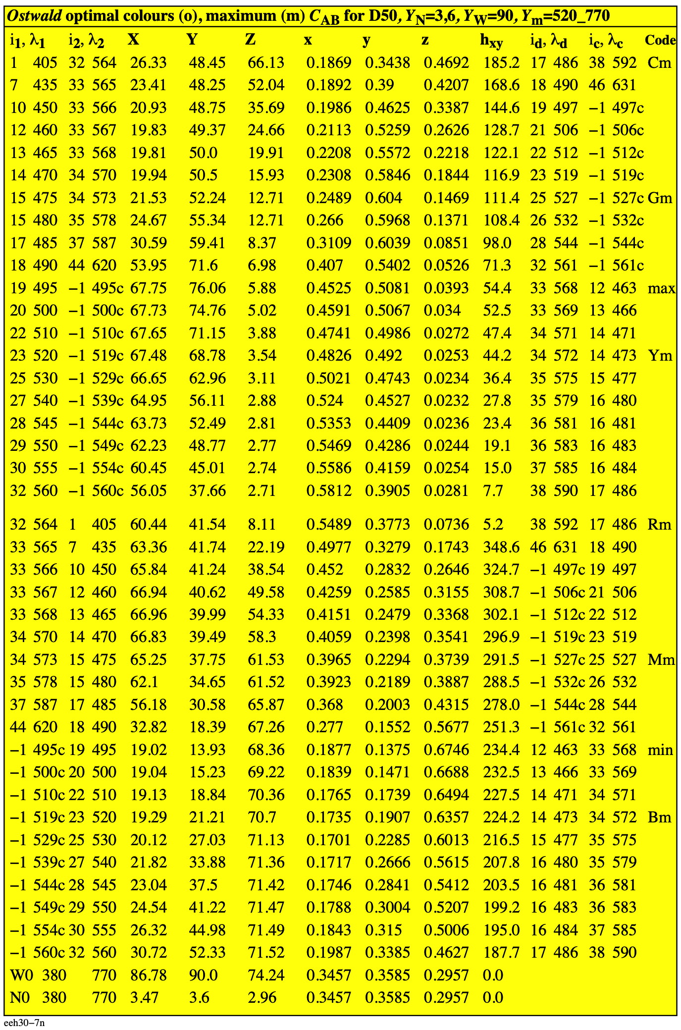
Figure 4.22-1: Colorimetric data of the Ostwald colours with wavelength limits and dominant wavelength
For the download of this figure in the VG-PDF format, see eeh30-7n.pdf.

The wavelenght on the purpur line are described with a "c=complementary to illuminant E".

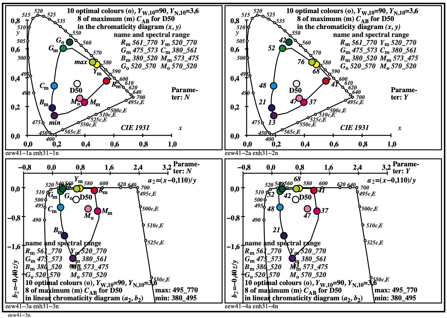
Figure 4.22-2: Colorimetric data of the Ostwald colours in different chromaticity diagrams
For the download of this figure in the VG-PDF format, see eew41-3n.pdf.

The Ostwald colours are specified by a name on the left side and by the tristimulus value Yo on the right side, and similar in Fig. 4.22-3.

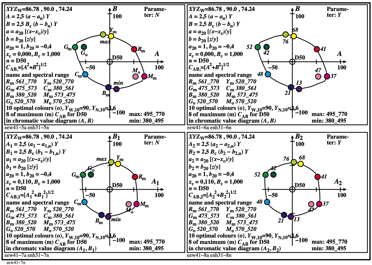
Figure 4.22-3: Colorimetric data of the Ostwald colours in different chromatic value diagrams
For the download of this figure in the VG-PDF format, see eew41-7n.pdf.

All Ostwald colours (o) of a colour half have different tristimulus values Yo, see Fig. 4.22-4.

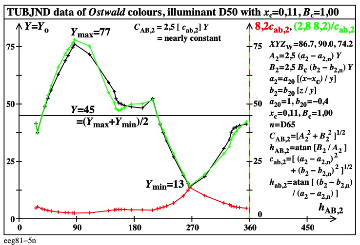
Figure 4.22-4: Tristimulus value Y=Yo of Ostwald colours (o) for the CIE standard illuminant D50
For the download of this figure in the VG-PDF format, see eeg81-5n.pdf.

However, the two chromatic values A2 and B2 produce approximately the same radial chromatic value CAB,2 for any hue and any adaptation, see Fig. 4.22-5.

Figure 4.22-5: Chromatic values A2 and B2 of Ostwald colours (0) for D50 with a nearly constant radial chromatic value CAB,2
For the download of this figure in the VG-PDF format, see eeg81-5n.pdf.

4.23. Constant radial chromatic values Cro of Ostwald colours for a wide range of chromatic adaptation between 6500K and 3000K.
All Ostwald colours (o) of a colour half have approximately equal radial chromatic values Cro. As example the values and equations are given for the CIE standard illuminant D50, see Fig. 4.23-1.

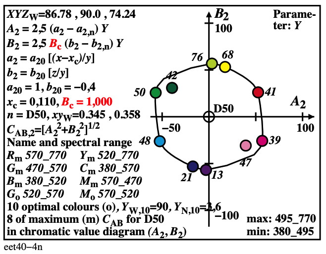
Figure 4.23-1: Calculation of radial chromatic values Cro of Ostwald colours (o) for the CIE standard illuminant D50
For the download of this figure in the VG-PDF format, see eet40-4n.pdf.

The mate surface colour range is limited to the range 3,6 <= Y <=90, see for example ISO/IEC 15775:2022 or ISO 9241-306:2019. Therefore the Ostwald colours are calculated for the same range.

For White the tristimulus value it is YW=90 and not 100. For Yellow the tristimulus value is YYellow=77 and the tristimulus value for Blue is YBlue=13. The tritimulus values of Yellow and Blue add to 90. The CIE chromaticity (x, y)W = (0,345, 0,358) does not change by the normalisation to the value 90 instead of 100.

The tristimulus-value ratio YYellow : YBlue = 77 : 13 = 6:1 is approximately constant for D50, and for all other Planck (Pxx) and Daylight (Dxx) illuminants according to ISO/CIE 11664-3:2019 Colorimetry - Part 3: CIE tristimulus values.

For the radial chromatic values Cro of the Ostwald colours (o) for the CIE standard illuminants D65, D50, A00, and the Planck illuminant P40 (4000K) with colour temperatures between 6500 K and 3000 K, see Fig. 4.23-2.

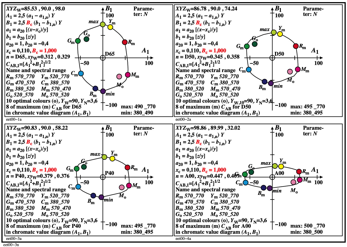
Figure 4.23-2: Colorimetric data of the Ostwald colours for D65, D50, A00 and P40 in the chromatic value diagram (A1, B1).
For the download of this figure in the VG-PDF format, see eet00-3n.pdf.

Different constants Bc between 0,8 and 2,5 change the chromatic values (A1, B1) to the chromatic values (A2, B2). The radial chromatic values Cro = CAB,2,o are approximately equal for all Ostwald colours.

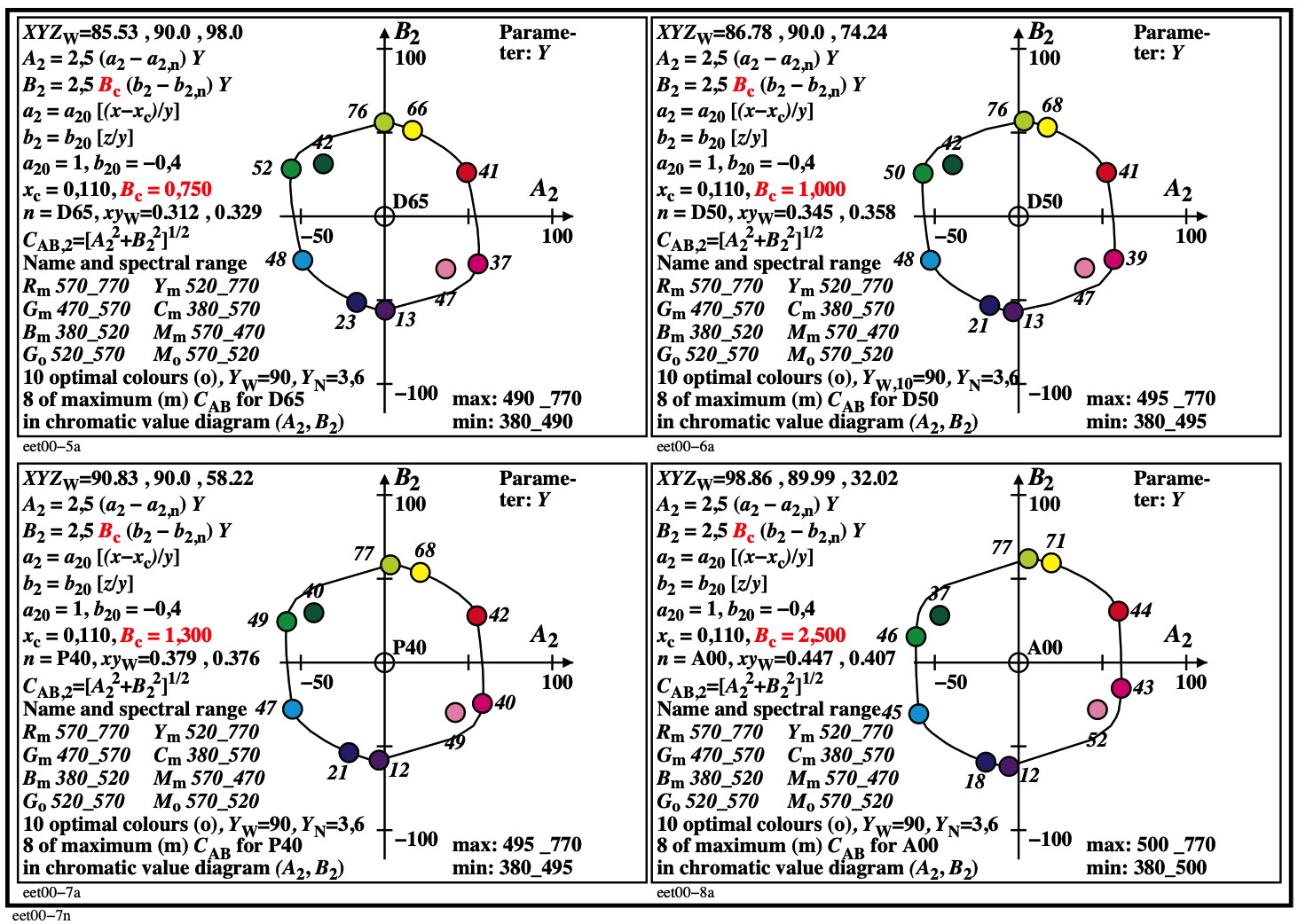
Figure 4.23-3: Colorimetric data of the Ostwald colours for D65, D50, A00 and P40 in the chromatic value diagram (A2, B2).
For the download of this figure in the VG-PDF format, see eet00-7n.pdf.

The colorimetric data of the Ostwald (o) colours for the 4 illuminants of Fig. 4.23-3 and all Planck illuminants between 6500 K and 3000 K have approximately equal radial (r) chromatic values Cro = CAB,2,o in the chromatic value diagram (A2, B2).

For all illuminants the CIE XYZxy data are different. All equations in Fig. 4.23-3 include only one parameter Bc. This parameter changes with the colour temperature between about 0,80 for 6500 K and 2,5 for 3000 K. This change is approximately a linear function of the CIE tristimulus values Z for both the eight illuminants Pxx and Dxx.

The hue angles are approximately equal for all Ostwald (o) colours (RYGCBM)m in Fig.4.23-3. The hue angles hAB,2 are approximately 30, 90, 150, 210, 270, 330 degree for the wavelength limits given in Fig. 4.23-3.

Additional Figures (only for download) show the above properties for the radial chromatic values Cro of the Ostwald colours (o) for 8 illuminants of both Planck and Daylight with colour temperatures between 6500 K and 3000 K.
For the download of these two figures in the VG-PDF format, see
http://farbe.li.tu-berlin.de/eet3/eet3l0np.pdf and http://farbe.li.tu-berlin.de/eet4/eet4l0np.pdf.

4.24. Improvement of colour-difference formula LABJND 1985 to TUBJNDs 2023 for chromatic colours with phsychophysical data.
CIE 230:219 Validity of colour difference formulae for small colour differences compares the performance of the colour difference formulae CIELAB, CMC, CIE94, CIEDE2000, and LABJND85. Out of 8 CIE datasets for small colour diferences and adjacent colour samples, the performance is best for LABJND in 5 of 8 cases, and best in one case of the 8 datasets for CIELAB, CMC and CIEDE2000.

The colour-difference formula LABJND 1985 of CIE 230:2019 includes chromaticity coordinates (a, b). Therefore the achromatic colour difference is extended by chromatic components. Experimental data for achromatic and chromatic thresholds are shown in Fig. 4.24-1.

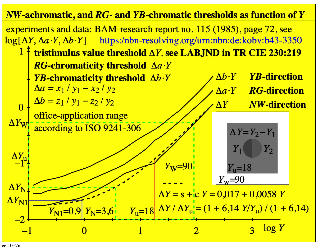
Figure 4.24-1: Achromatic and chromatic thresholds as function of Y.
For the download of this figure in the VG-PDF format, see eeg10-7n.pdf.

The chromaticity coordinates (a, b) defined in Fig. 4.24-1 are used for the colour difference formula LABJND in Fig. 4.24-2.

Figure 4.24-2: Chromatic values [(a" - a"n) Y] for D65 are the basis for the chromatic colour difference.
For the download of this figure in the VG-PDF format, see eeg11-3n.pdf.

For a constant Y value, and for example with an increasing chromaticity difference a - an, the difference of the chromatic value [(a - an) Y] decreases by the radial scaling factor sr = (1 + 0,5 |a - an| ).

The radial scaling factor sr increases for a threshold the chromaticity difference in the radial (r) direction for any hue. This is known from the colour difference formula CIEDE2000, the MacAdam ellipses and the chromatic threshold experiments of Richter (1995, pages 83-100), see the book http://color.li.tu-berlin.de/BUA4BF.PDF.

This book shows on page 85 for colours of equal Y, and for chromatic thresholds an increase of the chromaticity difference |a - an| for reddish and greenish colours, see Fig. 4.24-3.

Figure 4.24-3: Increase of the chromaticity difference |a - an| for equal chromatic thresholds, and for constant Y.
For the download of this figure in the VG-PDF format, see een10-7a.pdf.

In CIE 230 the scaling factor sr is defined as independent of hue, and uses not the different Y values of the Ostwald colours.

The hue dependent properties of different antagonistic pairs of Ostwald colours are shown in Fig. 4.24-4.

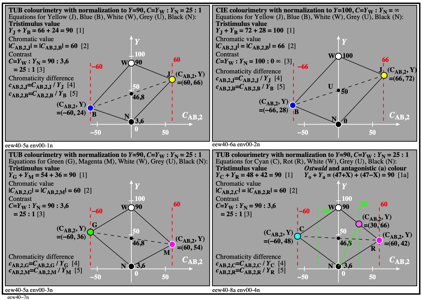
Figure 4.24-4: Different hue planes with the antagonistic Ostwald colour of antagonistic values Y which add to the value Y = 90.
For the download of the the figure in the VG-PDF format, see
eew40-7n.pdf

The radial chromatic values of all antagonistic Ostwald colours have the value Cro = CAB,2,o = 60. This leads to the antagonistic equation
cAB,2,o = 60 Yo [1]

Instead of the hue independent radial scaling factor sr a hue dependent radial scaling factor srh is used in Fig. 4.24-5.

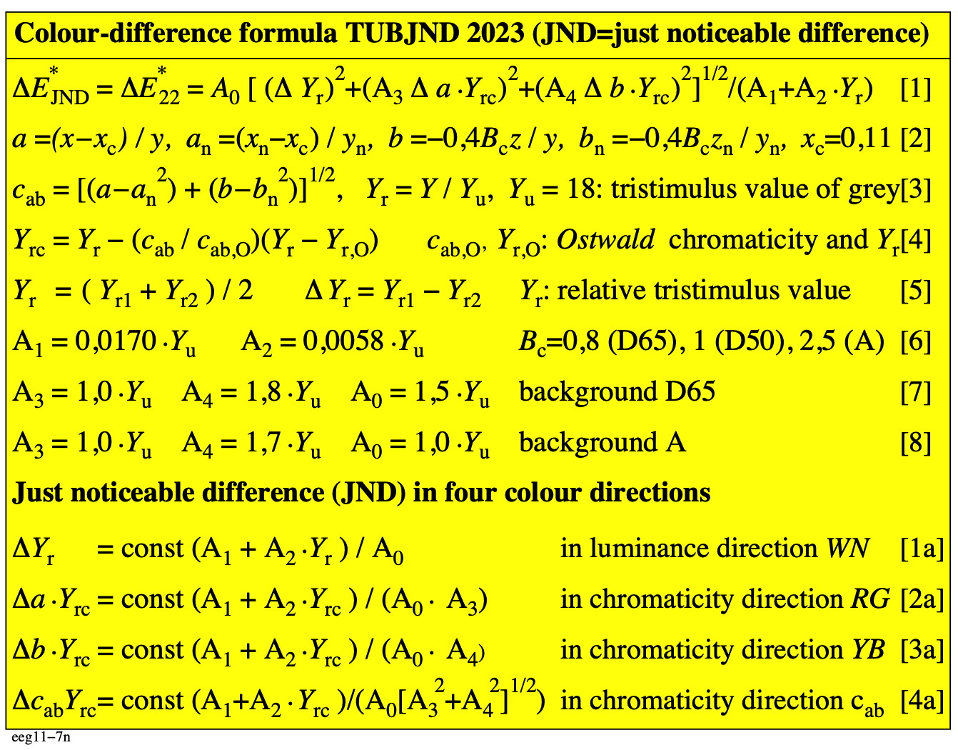
Figure 4.24-5: Chromatic values [(a - an) Yro] are the basis for the colour difference formula TUBJND 2023
For the download of this figure in the VG-PDF format, see eeg11-7n.pdf.

On can compare the chromatic values of the colour-difference formulae LABJND 1985 and TUBJND 2023:
compare LABJND 1985 in Fig. 4.24-2: |a" - a"n| Y with a" = an +(a - an)/(1+0,5|a-an|) and a = x/z

compare TUBJND 2023 in Fig. 4.24-5: |a - an| Yrc with Yrc = Yr - (a/ao) (Yr - Yro) and a = (x - 0,11) / y.

In LABJND 1985 a is changed to a".
In TUBJND 2023 Y is changed to Yrc (includes Ostwald colour data).

The colour-difference formula TUBJND 2023 uses the relative tristimulus values Yro of the Ostwald colours, see Fig. 4.24-5.

One can consider the equation
cAB,2,o = 60 Yo [1]

Then there are alternate versions of equation [4] in Fig. 4.24-5 without the trstimulus value Yo of the Ostwald colours and only with the chromaticity cAB,2 of any colour and the chromaticity cAB,2,o of the Ostwald colours.

Different versions of TUBJND 2023 are under consideration. The performance of LABJND 1985 in CIE 230 may increase by the use of the formula TUBJND 2023 for the defined CIE datasets for small and larger clour differences
For all experimental data of thresholds dL as function of Y the contrast Y/dY = L/dL can be calculated, see Fig. 4.24-5.

Figure 4.24-4: Luminance contrast L/dL for adaptation to surrounds in the luminance range 0,1 cd/m^2 <= Lu <= 1000 according to Lingelbach.
For the download of this figure in the VG-PDF format, see een40-2a.pdf.

In offices the surround luminance is Lu = 142 cd/m^2. This luminance corresponds to the illuminance 500 lux recommended in ISO/CIE CD 8995-1 Lighting of work places — Part 1: Indoor. We can assume, that the maximum contrast L/dL is reached at the surround luminance. In Fig. 4.24-4 this is nearly true for the surround luminance in offices.

Remark: The maximum contrast is higher for a lower luminance and lower for a higher luminance. This psychophysical property of Fig. 4.24-4 is also known from physiological experimental data, and will be discussed further in section 4.

For achromatic colours the maximum contrast is usually reached at the achromatic surround.

For chromatic colours the maximum contrast is usually reached at the Ostwald colour with the tristimulus value Yo and the radial chromaticity cab,o. For a lower radial chromaticity compared to cab,o, the maximum contrast is at the tristimulus value Yrc, see equation [4] in Fig. 4.24-3. The value of Yrc is between the tristimulus values of the Ostwald (o) colour and the achromatic surround (u). The value of Yrc is in the range
Yo <= Yrc <= Yu.

It is often appropriate to use a log instead of a linear scale for the contrast L/dL. This may show potential properties of the experimental data, see Fig. 4.24-5.

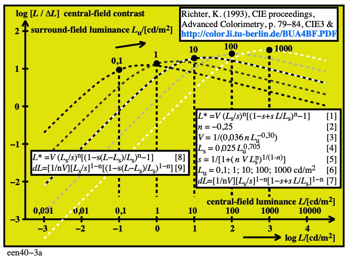
Figure 4.24-5: Luminance contrast log[L/dL] for the surround luminance in the range 0,1 cd/m^2 <= Lu <= 1000 according to Lingelbach
For the download of this figure in the VG-PDF format, see een40-3a.pdf.

The log output shows a slope near 1 in the dark range and a slope -1/3 in the light range compared to the surround. The slope in the light range depends to a large degree on the viewing time of the two adjacent samples. The slope changes from -1 to 0 for very short (<0,1s) to long viewing times (> 25s) by local adaptation.

The experimental viewing time for the thresholds of Lingelbach was 0,4s. The viewing time of the thresholds of the data of CIEDE2000 may be larger and therefore the slope is more near the value 0, for example near -1/6.

4.25. Lower and higher colour metrics with spectral sensitivities for elementary colours.

from RGB_CMYD_19.PDF produced from RGB_CMYD_42.fm
MG480-7N 2x2, Fig. 4.25-1
MG481-7N 2x2, Fig. 4.25-2
MG030-8N, Fig. 4.25-3
MG031-1N, Fig. 4.25-4
MG031-3N, Fig. 4.25-5
MG031-4N, Fig. 4.25-6

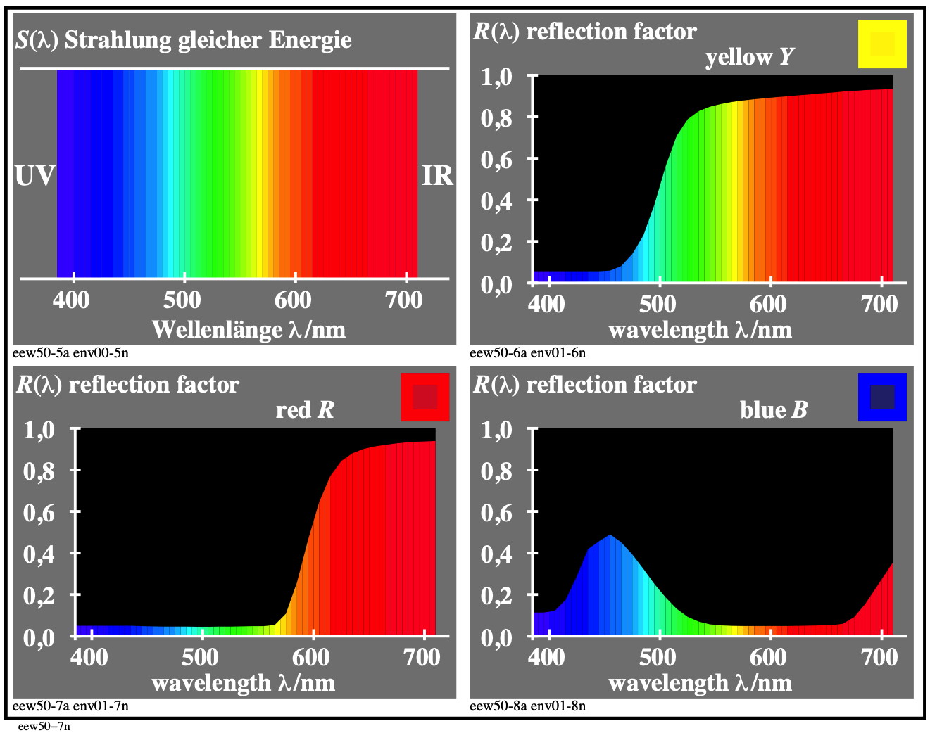
Bild 4.25-1: Text.
For the download of this figure in the VG-PDF format, see
eew50-7n.pdf

Bild 4.25-2: Text.
For the download of this figure in the VG-PDF format, see
eew51-3n.pdf

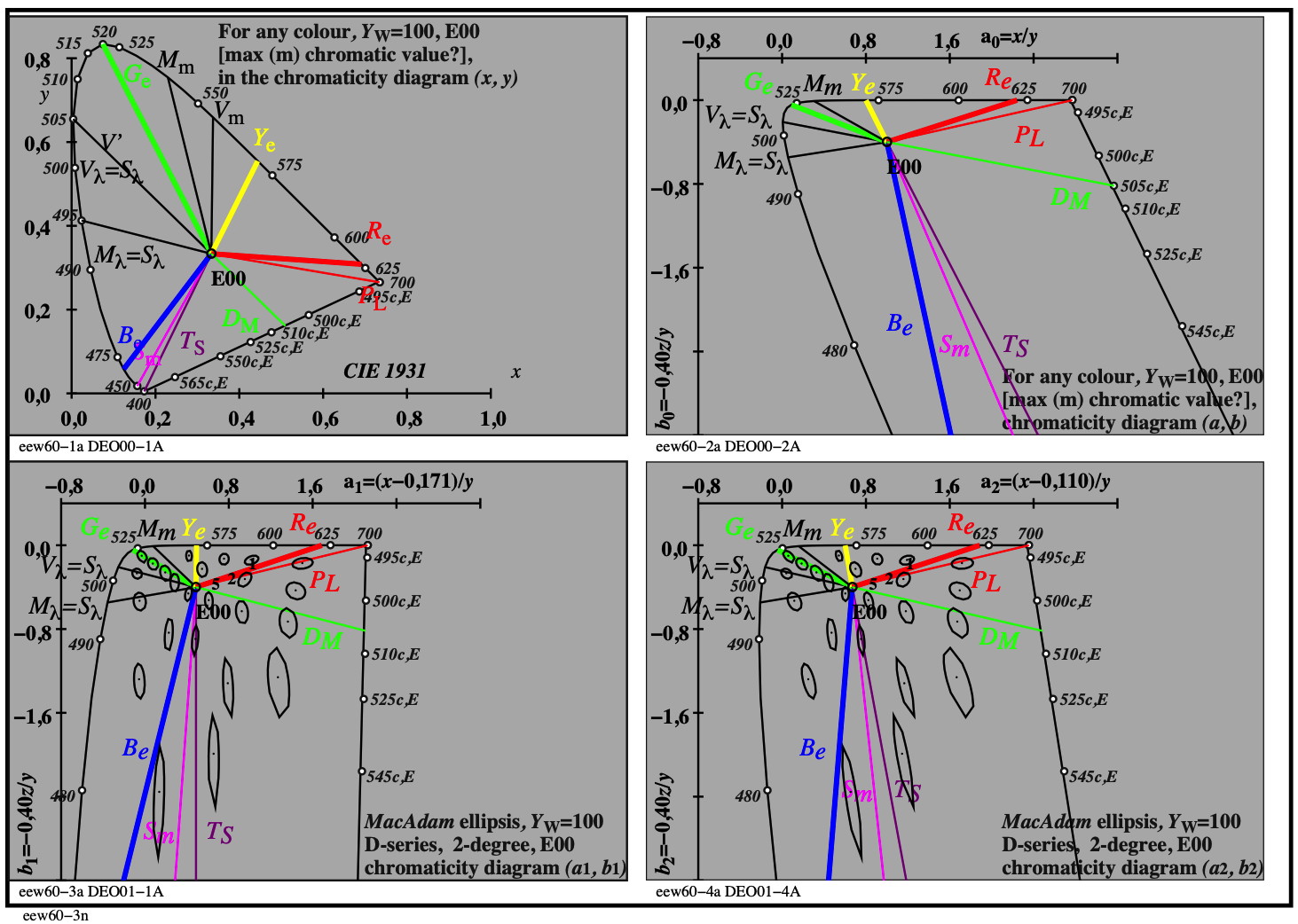
Bild 4.25-3: Text.
For the download of this figure in the VG-PDF format, see
eew60-3n.pdf

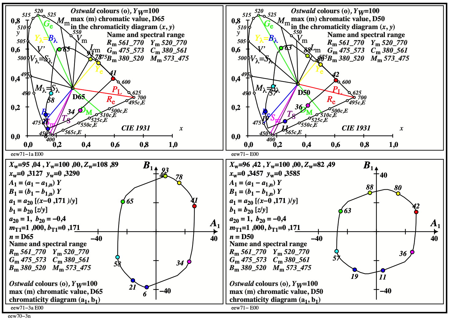
Bild 4.25-4: Text.
For the download of this figure in the VG-PDF format, see
eew70-3n.pdf

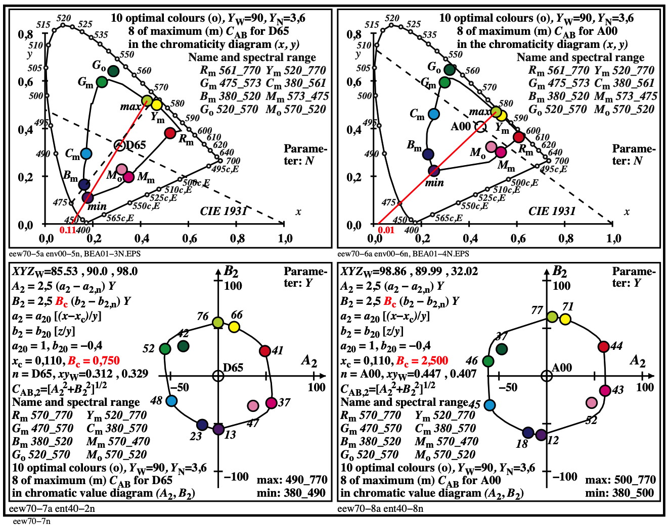
Bild 4.25-5: Text.
For the download of this figure in the VG-PDF format, see
eew70-7n.pdf

4.26. Atagonistic cone sensivity and models for summation and difference

This section includes a revision of a paper presented at the AIC conference in Jeju/Korea, 2017, see a draft: AIC17.PDF.
For the original AIC version, see AIC 2017, 13th Congress, paper OS07_6,
Colour Vision Properties of Surface Colours based on complementary Optimal Colours
Klaus Richter (Berlin University of Technology, Germany), Tuesday, 17th October 2017, see
https://aic-color.org/publications-proceedings.
For this section the references [1] to [7] are listed at the end.

Introduction.
There are different colour vision properties for related surface colours and unrelated colours in lighting technology. This paper studies special surface colours which are complementary optimal colours of a colour half and which are called Ostwald colours.

The spectral reflection on any Ostwald colour has the value one for a colour half and zero for the other half. The spectral wavelength limits of these colour halves are located on a line in the CIE (x, y) chromaticity diagram through the chromaticity (xn, yn) of or near CIE illuminant D50 which is a natural achromatic illuminant compared to the bluish CIE illuminant 65 and the yellowish CIE illuminant A. For D50 the Ostwald colours are placed approximately on a circle in a chromatic value diagram (see [1], Table 3 and Fig. 58??? for D65, the larger yellow blue extension reduces for D50, see Fig. 4.26-1c in the following).

Theory and experimental results
BE640-4A_1, Fig. 4.26-1a
BE640-5A_1, Fig. 4.26-1b
BE640-6A_1, Fig. 4.26-1c
Fig. 4.26-1a to c: HPE-cone sensitivities and parable functions with maximum values at 570, 540, 430nm
The cone sensitivities, the cone excitations, and the tristimulus value excitations are modeled by parables as function of wavelength. Fig. 4.26-1b is based on this model and allows to understand the existence of elementary colours and their spectral distribution. Fig. 4.26-1c shows the chromatic values of the Ostwald colours. The chromatic value A1 is based on the colour confusion lines of tritanopic observers.

The Fig. 4.26-1a to c show the cone sensitivities LMS which are calculated by the Hunt-Pointer-Estevez (HPE) transformation from the CIE spectral tristimulus values. The transformation equations are given in Fig. 4.26-1a. The data are still used in a new CIE Technical Report [2]. Many books on colorimetry propose similar peak values, for example the data 564, 534, and 420 nm of Oleari in [3, page 82]. The dashed lines in colour & black model the three cone sensitivities l(lambda), m(lambda), and s(lambda) by three parable functions in log units. In the short wavelength range below 530 nm the s(lambda) sensitivity is reduced by the eye media in the fovea, see [3, Fig. 5.4].

BE641-7A_1, Fig. 4.26-2a
BE641-8A_1, Fig. 4.26-2b
BE640-7A_1, Fig. 4.26-2c
Fig. 4.26-2a to c: CIE spectral tristimulus value and cone excitations
The Fig. 4.26-2a to c show excitations of the CIE tristimulus values X and Z and the L cone. The excitation is the ratio of the value and the tristimulus value Y. Similar the ratio of the tristimulus values X/Y, Z/Y, and L/Y can be used. The Y value is a linear transformation of the cone values L and M. Instead of the tristimulus values the spectral values are used in Fig. 4.26-2a to c. Fig. 4.26-2c may not be useful for applications.

BE860-1A, Fig. 4.26-3a
BE860-3A, Fig. 4.26-3b
BE860-5A, Fig. 4.26-3c

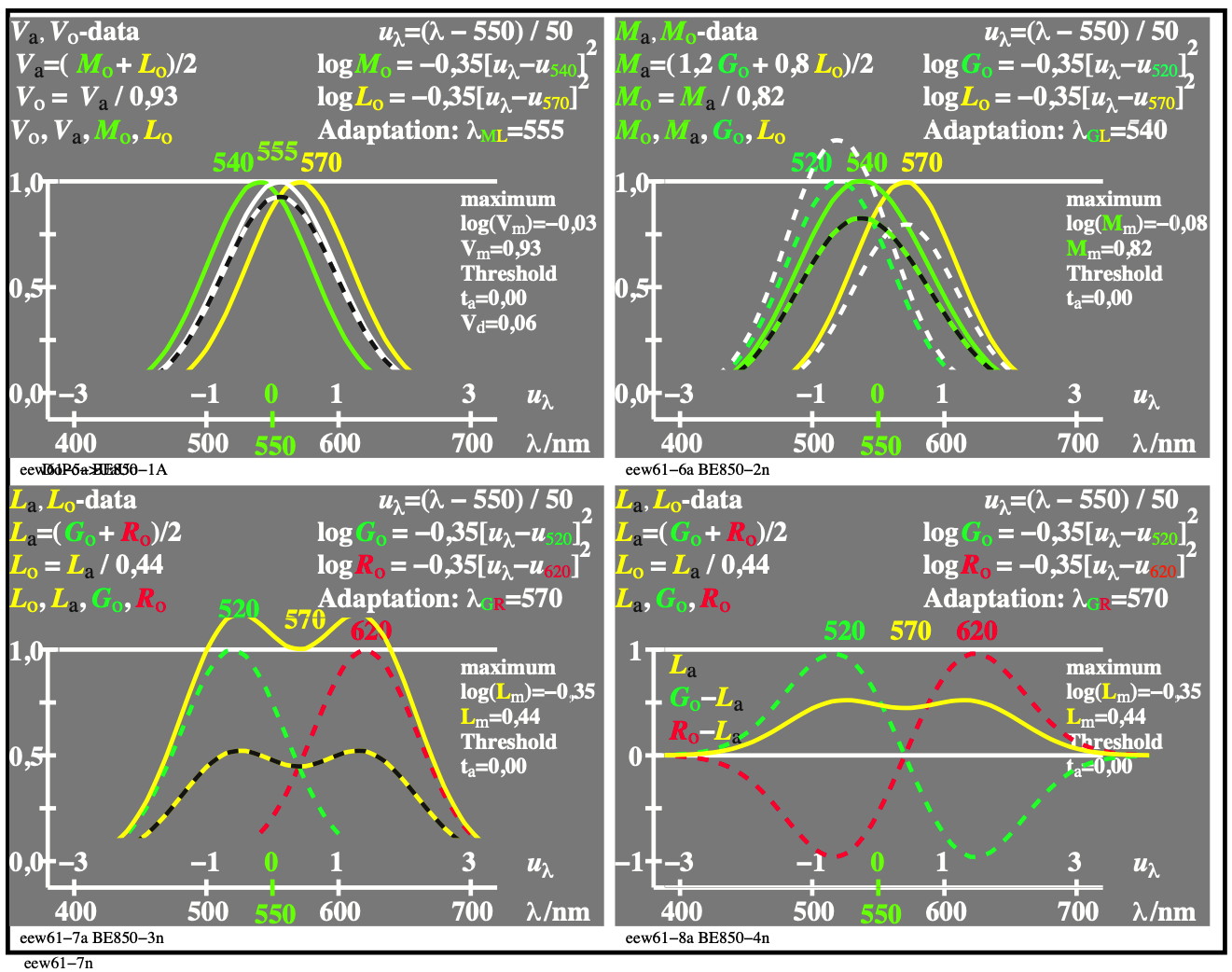
Bild 4.26-1: Text.
For the download of this figure in the VG-PDF format, see
eew61-7n.pdf

Bild 4.26-2: Text.
For the download of this figure in the VG-PDF format, see
eew21-3n.pdf

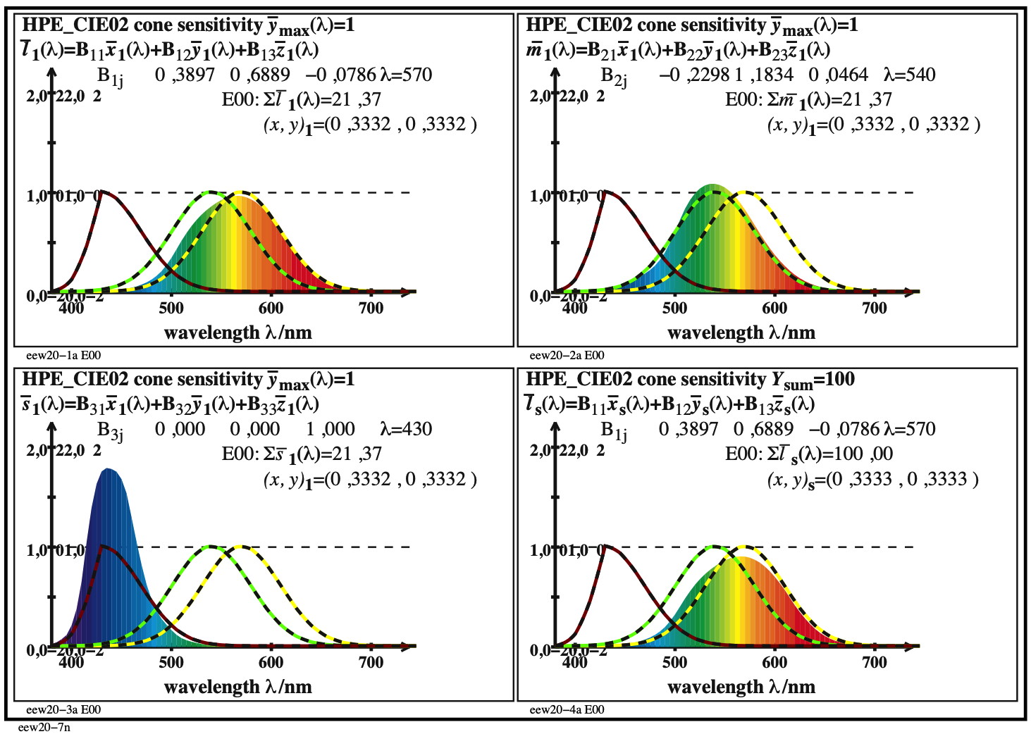
Bild 4.26-3: Text.
For the download of this figure in the VG-PDF format, see
eew20-3n.pdf

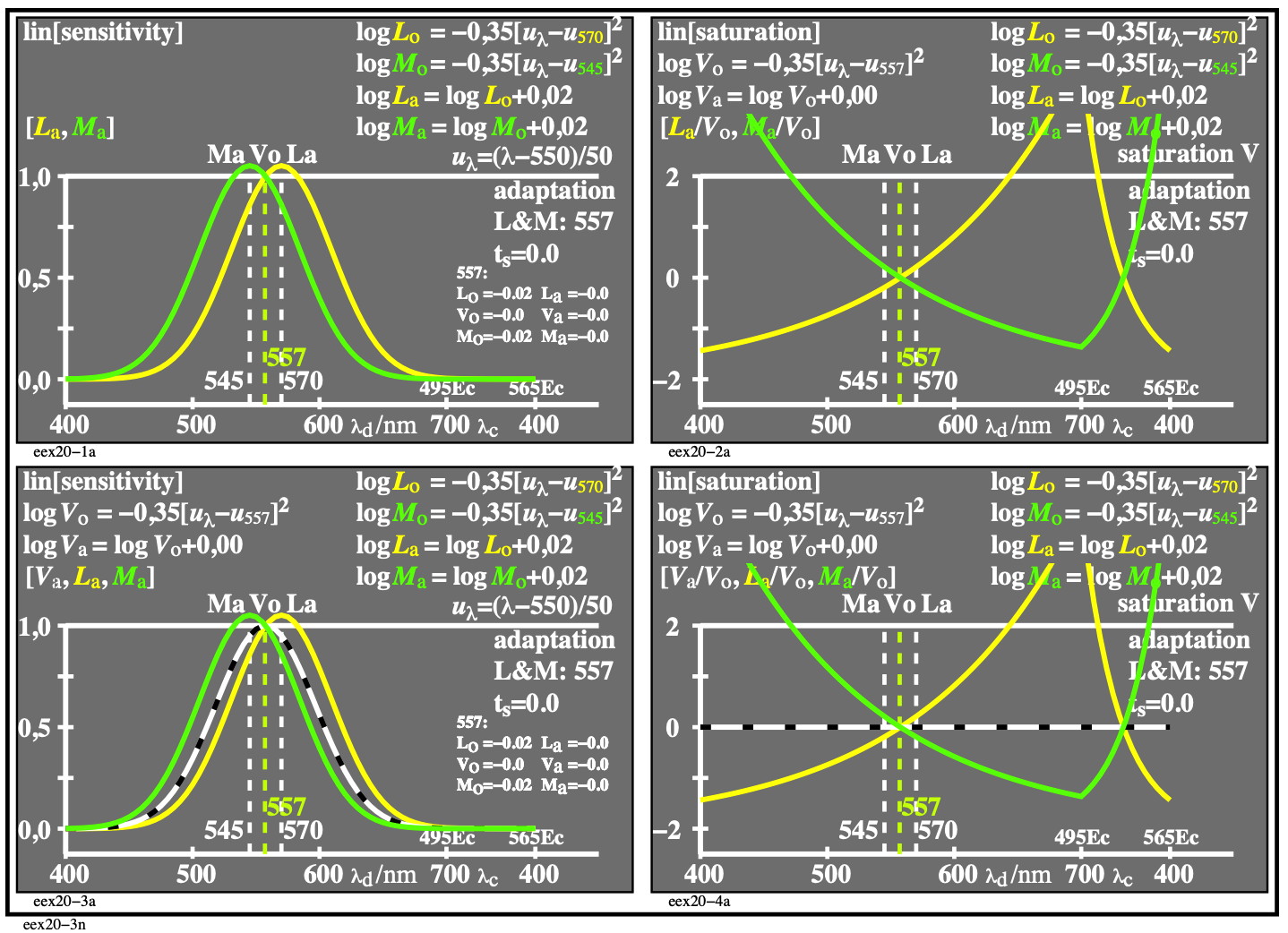
Bild 4.26-4: Text.
For the download of this figure in the VG-PDF format, see
eex20-3n.pdf

Bild 4.26-5: Text.
For the download of this figure in the VG-PDF format, see
eex21-3n.pdf

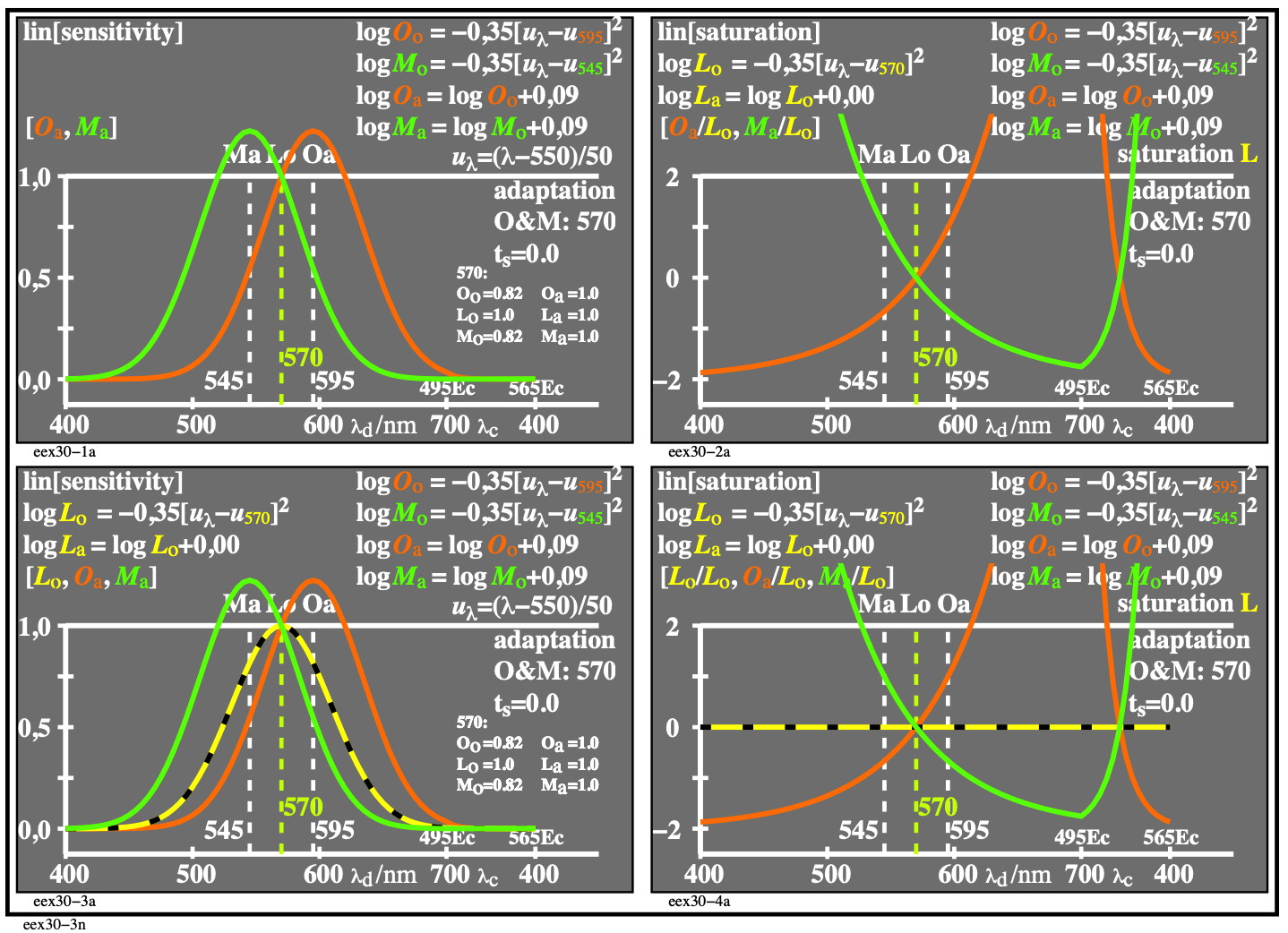
Bild 4.26-6: Text.
For the download of this figure in the VG-PDF format, see
eex30-3n.pdf

Bild 4.26-7: Text.
For the download of this figure in the VG-PDF format, see
eex31-3n.pdf

Fig. 4.26-2a to c: Logarithmic sum and differences of the spectral cone sensitivities
The Fig. 4.26-2a to c show example calculations of the sum and differences of the spectral cone sensitivities L and M.

The peak values of L (570 nm, yellow curve) and M (540 nm, green curve) have a difference of 30 nm. The yellow and green colour is used here to indicate that the peak value is in the yellow or green spectral range. The logarithmic sum and for example a linear sum differs by only 1% near 400nm and 700nm [3, Fig. 4-36]. The threshold value is 2% compared to the maximum value for surface colours, see [3, Fig. 6.17].
Therefore a decision of a linear or logarithmic sum is not possible in the case of surface colours. There is a long expert discussion about the ratio of the weighting factors. The ratio 1:1 is used in Fig. 4.26-3c and the ratio 1:2 is used in the HPE transformation. Recent studies show that there are large individual variations in the relative numbers of cone types and their distribution in the retina [3, section 5.4.6].

A logarithmic calculation in Fig. 4.26-3a to c allow to calculate the same shape for these experimental variations in cone distributions. Equations (1) to (5) show examples used in the plots of Fig. 4.26-3a to c.

logVa = 0.5[logMo +logLo] (1) or
Va =(Mo xLo)0,5 (2)
or logMo = 2logVa –logLo (3) with
log Vo = log Va + 0.03 (4)

The cone excitation is the logarithmic (linear ratio) or the logarithmic difference
log (Mo/Va) = logMo - logVa (5)

If the peak values are normalized to one the index (o) is used. The sum and differences produce peak values below one and in this paper then the index (a) is used. The symbols Va (white-black curve) and Vo (white curve), see Fig. 4.36-3a are proportional to the luminous tristimulus value Y. Va(λ) is smaller compared to Vo(λ) by the factor 0,97 in logarithmic units and 0,93 in linear units. See also more values in Fig. 4.26-3b and c.

In Fig 2f-3a the functions Va(lambda) and Vo(lambda) are calculated according to equation (1).
Similar in Fig. 4.26-3b the La(lambda) and Lo(lambda) functions are calculated from calculated sensitivities Ro(lambda) and Go(lambda). All calculated sensitivities are shown by dashed curves. Fig. 4.26-3c uses the red and green colours according to the location in the spectral range.
Fig. 4.26-3c is similar with peak values 570, 520, and 470 nm. These are the peak values of the spectral elementary colours, for example the elementary (e) green Ge as neither yellowish nor bluish.

BE860-2A, Fig. 4.26-4a
BE860-4A, Fig. 4.26-4b
BE860-6A, Fig. 4.26-4c
Fig. 4.26-4(a, b, c): Cone excitation as logarithmic ratio of the spectral or calculated cone sensitivities
The Fig. 4.26-4 show the logarithmic ratio of the real or calculated cone sensitivities in Fig. 4.26-4a to b as function of wavelength according to equation (5). The slope increases with the difference of the peak values.

BE830-3A, Fig. 4.26-5a
BE830-4A, Fig. 4.26-5b
BE830-8A, Fig. 4.26-5c
Fig. 4.26-5(a, b, c): Sensitivities M (540nm), L (570nm), and O (600nm) on a linear ordinate.
Fig 2f-5a shows a linear ordinate scale for three sensitivities Mo, Lo, and Oo. La is calculated by the logarithmic sum of Mo and Oo.

Fig. 4.26-5b shows the linear differences of Fig. 4.26-5a. For the sensitivity difference Oo(lambda) - La(lambda) a dashed curve in red is used because the sensitivity Oo(lambda) is a calculated sensitivity. Together with similar functions in the blue part around 470 nm (of smaller values?) the hue appearance in the spectral range according to the elementary (e) colours Be, Ge, Ye, and Re can be described.

BE321-1A_1, Fig. 4.26-6a
BE321-2A_1, Fig. 4.26-6b
BE321-3A_1, Fig. 4.26-6c
Fig 2f-6(a, b, c): Peak sensitivities Lm, Mm, Sm , confusion lines of PL, DM, TS observers, and elementary hues.
Fig. 4.26-6a shows the location of the peak sensitivities Lm, Mm, Sm, the confusion lines of PL, DM, TS observers, the elementary hues Be, Ge, Ye, and Re and all Ostwald colours in the CIE chromaticity diagram (x, y).

Fig. 4.26-6b and c show the chromatic value of the Ostwald colours under an illumination which appears natural white. The CIE standard illuminant D50 is near the natural white. The CIE daylight D65 (CCT 6500K) appears bluish and a tungsten light (CCT 3000K) is yellowish. An illumination with a linear change of the CIE illumination E(lambda) of equal energy as function of lambda appears similar to D50.

The spectral distribution is P(lambda) = lambda/560nm E(lambda), and is called P00 in this paper. With the linear equations given in Fig. 4.62 and 6c the antichromatic Ostwald colours have antichromatic colour values and are located approximately on a circle. The chromaticities (x, y) are shown in Fig. 4.61. The CIE tristimulus values differ by a factor 8 (between 88 and 11, see parameter Y in Fig. 4.26-6b or c. Therefore the tristimulus value excitation difference a - an = x/y - xn/yn and similar for b - bn is by a factor 8 smaller for yellow Ye compared to blue Be.

DM100-3N_7, Fig. 4.26-7a
DM101-5N_7, Fig. 4.26-7b
Fig. 4.26-7a, b: Chromatic values A0, B0, C0,AB and chromaticities (a, b) of Ostwald optimal colours.
The Fig. 4.26-7a shows the chromatic values A0, B0, and the chromaticities (a0, b0) of the Ostwald-optimal colours. The chromaticity difference of any colour compared to the achromatic colour W1 in Fig. 4.26-19 is by a factor 8 different. If the difference is small the Y values is high and vice versa.

In Fig. 4.26-7b the chromatic value C0,AB is approximately independent of hue and of the Y value for the antichromatic Ostwald optimal colours.

Results and discussion
The confusion lines TS and PL of the Tritanope (T) and Protanope (P) observers with missing L and S cones connect the achromatic and the chromaticity of 400 nm and 700 nm in Fig. 4.61. The TS line defines a basic chromatic value system (A1, B1), see Fig. 4.63, to produce equal chromatic values for the Ostwald colours. In Fig. 4.62 the system (A0, B0) produces a slightly less performance. However, (A0, B0) matches the property of CIELAB that elementary yellow and blue is located on the vertical axis and both red and green are shifted about 30 degree upwards compared to the horizontal axis. Therefore, for the description of the hue angles the linear chromatic value diagram (Ao, Bo) is similar to the cube root chroma diagram (a*, b*) of CIELAB because of similar hue angles for the elementary colours [5]. An application example is given in CIE R1-57 [6] which uses the Ostwald colours to describe the border between blackish and luminous surface colours.

Conclusion and development
All Ostwald colours have approximately the same chromatic value C0,AB, see Fig. 7a. For the Ostwald colours this is surprising because the tristimulus values Y and the tristimulus value excitations, for example x/y = X/Y vary by a factor 8. The equal chromatic values of the Ostwald colours in Fig. 4.63 are a basis for a colorimetric description of the experimental results of Holtsmark and Valberg [7]. The experimental equal colour threshold for all antichromatic optimal colours needs the equal chromatic values. A following paper will develop an improved colour metric for surface colours and will use cone and tristimulus value excitations.

Acknowledgement and remarks
I thank Thorstein Seim (Norway) for many proposals to improve the results on this paper. Most figures of this paper have a code of four letters, for example BE32, see Fig. 7. One can find this figure and many similar ones on a public university server
http://130.149.60.45/~farbmetrik/BE32/index.html or a copy (less actual) on the public server http://farbe.li.tu-berlin.de/BE32/index.html. Both servers include many additional references.

References of section 2f:
[1] Richter, Klaus, 2016, Colour and Colour Vision and Elementary Colours in Colour Information Technology, 85 pages (A5), (available in 5 languages), see
http://color.li.tu-berlin.de/color.
For an english version for the (mobile) display output, see
http:/standards.iso.org/iso/9241/306/ed-2/ES15.PDF.
This paper includes the printed achromatic and chromatic test charts with elementary colours according to ISO/IEC 15775:2022, see http:/standards.iso.org/iso-iec/15775/ed-2/en.

and according to ISO 9241-306:2018, Annex D, see for example test chart AE49 on
http:/standards.iso.org/iso/9241/306/ed-2/index.html.

[2] CIE 224:2017. Colour Fidelity Index for accurate scientific use.
[3] Oleari, Claudio, 2016, Standard Colorimetry, Definitions, Algorithms and Software, Wiley.
[4] Richter, Klaus, 1996, Computergrafik und Farbmetrik, Farbsysteme, see
http://farbe.li.tu-berlin.de/buche.html.

[5] Thorstein Seim, (2009), Reportership Report CIE R1-47, Hue angles of elementary colours, see (35 pages),http://web.archive.org/web/20160304130704/http://files.cie.co.at/526.pdf.

[6] Thorstein Seim, (2013), Reportership Report CIE R1-57, Border between Blackish and Luminous Colours, see (23 pages), http://web.archive.org/web/20150413002133/http://files.cie.co.at/716_CIE%20R1-57%20Report%20Jul-13%20v.2.pdf.

[7] Holtsmark, T. and Valberg, A. (1969), Colour discrimination and hue, Nature, Volume 224, 366-367.

4.27. Experimental results of Evans on blackness and the black threshold and comparison with the TUBLABs colour space.

Bild 4.27-1: Antagonistic Ostwald colouras in antagonistic hue planes with antagonistic Y values which add to the value Y = 90.
For the download of this figure in the VG-PDF format, see
eew51-7n.pdf

4.28: Relations of experimental data of Evans on colour appearance and the TUBLAB colour space.
The book of Evans on colour appearance (1973) includes many results on colours of cero greyess for achromatic and chormatic surrounds. A colorimetric model for the descriptions of his experimental results is mostly unknown.

Figure 4.28-1: Tristimulus value Yo as function of the hue angle hAB,2o of the Ostwald colours (o)
For the download of this figure in the VG-PDF format, see eeu00-1n.pdf.

The Yo function is shown as function of the dominant wavelength in Fig. 4.28-2.

Figure 4.28-2: Tristimulus value Yo as function of the dominant wavelength lambdado of the Ostwald colours
For the download of this figure in the VG-PDF format, see eea10-5n.pdf.

The output as function of the domiant wavelength looks very similar compared to the tristimulus value of cero greyness of the experimental results of Evans and Swenhold.

The crosses are the caculated data of the Ostwald optimal colours and are not the Go-data of Evans and Swenhold. A paper of Richter (1971) has tried to describe the Evans and Swenhold results and many others on colour appearance, see
Richter, K. (1971), Description of colour attributes and colour differences, in Proceedings of the Helmholtz Memorial Symposium on Color Metrics, AIC/Holloand, Soesterberg, p.134-146, see
https://aic-color.org/publications,
go to AIC 1971 to download the above paper of Richter, and related papers.

_________________________
For links to the main chapter E
Colour Metrics, Differences, and Appearance (2023), under work.
Content list of chapter E (links and file names use small letters), see
eea_s in English or ega_s in German.

This web page is since 2023 under work.
In future the figures and the text may be improved.

Link to the next topic (under work in 2023)
Title of part 4.3: Achromatic colour metric for a wide luminance range between the Low, Standard and High Dynamic Range (LDR, SDR, and HDR)
eea_s43 in English or ega_s43 in German.

-------
For the TUB start site (not archive), see
index.html in English, or indexDE.html in German.

For the TUB archive site (2000-2009) of the BAM server "www.ps.bam.de" (2000-2018)
about colour test charts, colorimetric calculations, standards, and publications, see
indexAE.html in English, indexAG.html in German.

For similar Information of the BAM server "www.ps.bam.de" from the WBM server (WayBackMachine)
https://web.archive.org/web/20090402212108/http://www.ps.bam.de/index.html