4.42. Colour stimuli and colour sensation for chromatic colours: mixing and antagonism
The most chromatic surface colours are the Ostwald colours. In many applications, three colour pairs Red-Cyan (R-C), Yellow-Blue (Y-B) and Green-Magenta (G-M) are used, see Fig. 4.42-1.
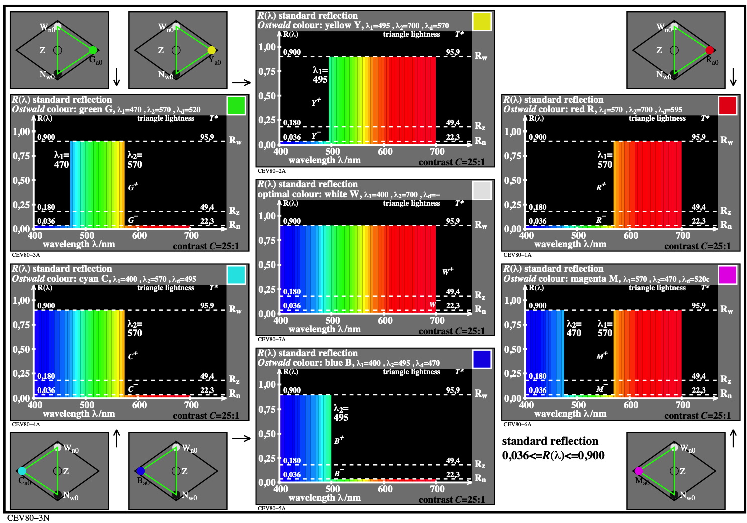
Fig. 4.42-1: Reflection as function of the wavelength for six Ostwald colours and the position of their mixed colours in different hue planes.
For the download of this figure in the VG-PDF format, see CEV80-3N.PDF.
The mixed colours are shown in a square at the upper right corner of the seven partial figures.
Fig. 4.42-1 shows the Ostwald colours and its reflections in a 6-step colour wheel RYGCBM. The values of the standard reflections RW of white, RU of medium grey U and RN of black (N=noir) are by a factor of 100 smaller than the standard chromatic values YW, YU and YN.
In the TUB model the white foot has the reflection RN=0,036. The middle grey has a reflection of RU = 0,180. The white has a reflection of RW = 0,900. The three values are shown in Fig. 4.42-1 by dashed lines.
0,2 <= Rr <=5 [3] or
-0,69 <= log Rr <= 0,69 [4].
The relative lightness function compared to the medium grey U is
L*TUBr = k log Rr with k = 40/log(5) = 57,22 [5]
This equation meets a standard goal of the TUB colour vision model.
Similar to the OSA-colour system, the relative lightness is zero for medium grey U and negative for darker colours and positive for lighter colours. The lightness L*TUBr is an S-shaped function and saturates below black N and above white W.
In the TUB model, the lightness values are therefore for white (W), grey (U), and black (N):
L*TUBr,W=40, L*TUBr,U =0 , L*TUBr,N =-40 [6]
If the value 50 for grey U is subtracted from L*CIELAB, the relative CIE lightness is:
L*CIEr = L*CIELAB - 50 [7]. The three values are:
L*r,W=45, L*CIEr,U =0, L*CIEr,N =-28. [8].
The symmetric relative lightness L*TUBr [5] is a logarithmic function.
4.43 Colour sensation for chromatic colours: mixture, signals and antagonism
For the calculation of the antagonistic signals R+ and R- and for the five hues YGCBM, the logarithmic relative reflections Rr = RW/RU and Rr = RN / RU are used, see Fig. c-1
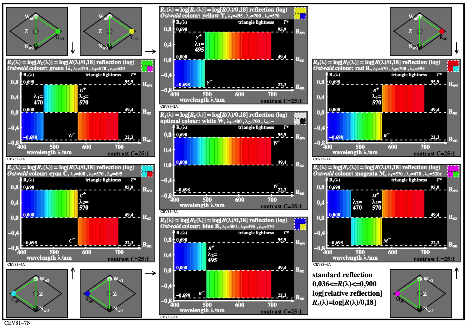
Fig. 4.43-1: Antagonistic signals R+ and R- of six Ostwald colours and their positions in different hue planes
For the download of this figure in the VG-PDF format, see CEV81-7N.PDF.
No physical reflection smaller than RN of black is used for the chromatic colour signals. We see a main feature: any reflection smaller than RN does not contain colour information, see Fig. 4.43-1. Therefore, the reflection range between 0 and RN is not used to calculate the colour values. This is a fundamental difference between the relative TUB and the CIE colourimetry.
For example, the relative CIE colourimetry of CIELAB includes the reflection part RrN = 0,036 down to the relative reflection Rr = 0,000. For matte samples, the limit value is RrN = 0,036. Similar glossy black samples may have a lower value Rr. In application, retro-reflective white samples may have a value Rr larger 1.
In the TUB model, the maximum reflection data of the colour pairs R-C, Y-B and G-M are the same and equal to the white reflection RW=0,900 with the relative reflection RrW=5. The chromatic values CA2B2 are the same and the tristimulues values Y differ. They have the highest value near Yellow and the lowest value near Blue, see the Y values in Fig. 4.43-1.
For example, the CIELAB chroma C*ab and the RG and YB components a* and b* of all Ostwald colour pairs differ. In the TUBr model, however, the chromatic values of the components RG and YB are, as expected, antisymmetric because they mix to a grey.
4.44. Equal chromatic values CA2B2 and equal hue-angle discrimination dhA2B2
For the Ostwald colours the CIE chromatic values were calculated for four different CIE illuminants, see Fig. d-1
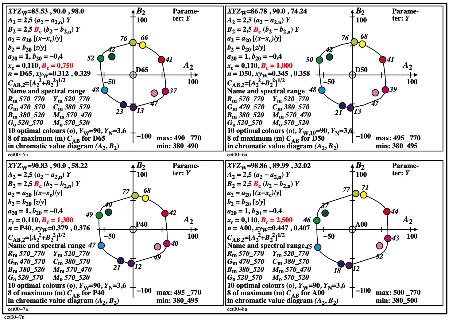
Fig. 4.44-1: Chromatic values of 6 Ostwald colours for CIE illuminants D65, D50, A, and E
For the download of this figure in the VG-PDF format, see eet00-7n.pdf.
The chromatic values CA2B2 are determined from the CIE values x, y, Y and an adaptation parameter Bc which is shown for D65, D50, P40, and A in the Fig. 4.44-1.
The chromatic-value components A2 and B2 have the same amount for all colour pairs. Therefore, the radial chromatic value CA2B2 is the same for all colour pairs. In addition, the radial chromatic value is also approximately the same for all Ostwald colours.
This property is expected according to the law of colour consistency for a change of the illuminant. Therefore all values of the TUB model are antagonistic and antisymmetric. Therefore, one can assume that equal hue-angle changes dhA2B2 produce the same visual differences.
For the Ostwald colour pairs the CIELAB chroma data a* and b* differ by a factor of 2 (not shown here). Therefore the CIELAB chroma values are not antagonistic, and are not antisymmetric. However, this are main properties for the linear chromatic values A2 and B2 of the TUB model.
Visual experiments may decide, if the linear chromatic values of the TUB model may also give a good description of the visual chroma.
If a nonlinear formula for the transfer from the chromatic value to the new chroma value is necessary, then again two equal chroma values are expected for antagonistic colours. For example the TUB model with linear chromatic values can be extended by a logarithmic transfer which may be linear for small chromatic and chroma values.
Remark:
Some wavelength boundaries of the Ostwald colours are slightly different compared to Fig.4b-1, 4c-1, and 4d-1. The wavelength limits change by 5 nm with the CIE illuminant, see in Fig. 4.43-1 the ranges after "max" right down for the CIE illuminants D65, D50, A and E.
4.45. Colour hue discrimination as function of the hue angle dhA2B2 and the wavelength dlambda
The spectral colour mixture produces the most chromatic surface colours, see Fig. 4.45-1
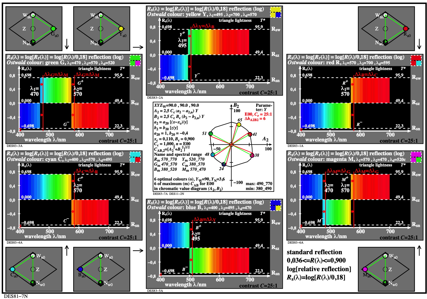
Fig. 4.45-1: Spectral and chromatic values of six Ostwald colours for the CIE illuminant E with hue discrimination as a function of the hue angle dhA2B2 for the contrast C = 25:1.
For the download of this figure in the VG-PDF format, see DES81-7N.PDF.
The colour mixtures are shown in the upper right corner for the six colours together with complementary colours.
According to the psychophysical experiments of Holtsmark and Valberg (1969), the threshold of the wavelength shift dlamdba of complementary optimal colours R-C, Y-B, and G-M is approximately the same, see the six Ostwald spectra. The shift dlamdba is experimentally smaller for the pair Y-B than for the other two pairs (not shown here).
In Fig. 4.45-1 it is assumed that the colour threshold (a Just Perceptible Difference JND) is about 6 degrees for the 6 colours of the Ostwald-colour circle. Therefore, about 60=(360/6) steps of the very chromatic Ostwald colour circle can be distinguished.
Fig. 4.45-1 shows in the middle part a hue-angle change dhA2B2 = 6 degrees due to red lines from the origin compared to the green lines. The six red lines correspond to six red lines in the six Ostwald spectra. The TUB model results in the same hue-angle shift dhA2B2 = 6 for all six Ostwald colours. This prediction is to be expected due to the approximately constant chromatic values for all shifts. The only slight change in lightness compared to the chromatic value may not affect the threshold.
Holtsmark and Valberg (1969) have used adjacent optimal colours in a white surround, and in a dark room. This white-black state can lead to a medium grey adaptation. For different adaptations, the value dlamda may only change by a constant factor. For purple Ostwald colours, the complementary wavelength dlamda1c and dlamda2c of Holtsmark and Valberg are given.
Holtsmark, T. and Valberg, A. (1969), Colour discrimination and hue, Nature, Volume 224, October 25, pp. 366-367.
4.46. Experiment for equal hue discrimination of complementary optimal colours
There is a visual phenomenon with complementary optimal colours produced by a positive and negative mask. A prism visually creates a similar distinction at corresponding locations within both spectra. This indicates a high symmetry in vision and is a basis for the TUB colour vision model. In addition, this leads to improved formulae for describing the colour threshold, see CIE 230:2019 entitled: Validity of Formulas for Predicting Small Colour Differences.
Optimal colours are produced by a mixture of all spectral colours between two wavelength limits, see Fig. 4.46-1.
Fig. 4.46-1: Complementary optimal colours produced by a positive and negative mask with a prism.
For the download of this figure in the tiff format, see SpektrumGrebe-ellis.tiff.
If the wavelength range for both the positive and negative mask is about 100 nm, we see in Fig. 4.46-1 (left) three primary colours O, L and V (orange red, leaf green and violet blue according to ISO/IEC 15775:2022) and im Fig. 4.46-1 (right) three complementary colours C, M and Y (cyan blue, magenta red and yellow).
The visual phenomenon arises, since the visual hue discrimination for the two colour series OLV and CMY for corresponding places is approximately the same. This applies approximately to each mask width for all positive and negative masks and therefore for all complementary optimal colours.
Holtsmark and Valberg (1969) measured the hue discrimination for optimal colours with a spectral colour integrator. In a white surround in a dark room with two identical masks, they have created two equal semi-circular central fields of about 2 degrees in diameter. The position of one mask had to be shifted until a hue threshold was visible. The same was repeated through an inverse mask and for six observers. The summary is in the statement:
The hue discrimination is approximate equal for a negative and positive mask.
The colour change is mainly defined by a constant hue angle shift, for example dhA2B2 = 6, see the chromatic values in Fig. 4.45-1. In the experiments of Holtsmark and Valberg, the chromatic values CA2B2 change with the gap width. Therefore, the experimental results of Holtsmark and Valberg are more general: All complementary optimal colours and not only complementary Ostwald colours produce the same experimental colour discrimination.
The TUB colour-vision model may form a basis for describing these additional experimental results. For this purpose, experimental results for the change of lightness and chromatic values as function of contrast are used in the following.
Acknowledgements:
I would like to thank Prof. Dr. Johannses Grebe-Ellis, the owner of the website http://www.experimentum-lucis.de for the permission to use in this work a figure of his website (which contains many more references).
4.47. Visible luminance range and nonvisible luminance in the black and white whole
The receptor responses and the discrimination by the TUBJND colour-vision model will be discussed for about 6 log units of luminance. New HDR displays may emit about 4 log units between 0,2 cd/m^2 and 2000 cd/m^2. Between the device White W and Black N the luminance ratio is then LdW : LdN = 10000 : 1. The luminance ratio of the mate surface colours White and Black is 90,9 : 3,6 = 25 : 1.
The very different luminance ratio for HDR displays and surface colour raises the question of the perceptive luminance ratio. In many cases the perceptive luminance ratio is limited to the ratio 25 : 1. However, by adaptation the perceptive luminance range can be shifted from a usually not visible Black Whole via the usual perceptive window to the usually not visible White Whole, see Fig. 4.47-1.
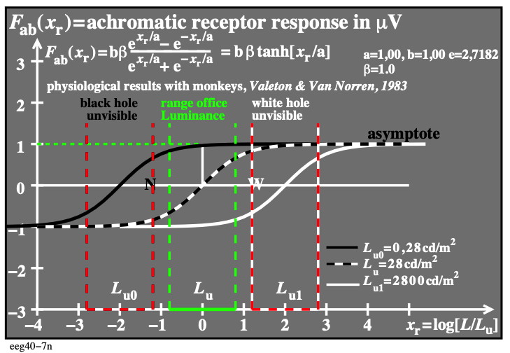
Fig. 4.47-1: Physiological achromatic receptor response of monkeys according to Valeton & Van Norren 1983
For the download of this figure in the VG-PDF format, see eeg40-7n.pdf.
Usually in vision there are also antagonistic (opponent) responses, see Fig. 4.47-2.
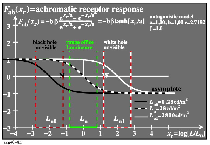
Fig. 4.47-2: Antagonistic Physiological achromatic receptor responses for three luminance adaptations
For the download of this figure in the VG-PDF format, see eeg40-8n.pdf.
For the usual luminance range in offices the receptor response and its derivation is shown. The response is S-shaped and the derivation is Gauss-shaped., see Fig. 4.47-3.
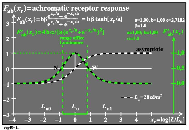
Fig. 4.47-3: Receptor response (S-shaped) and its derivation (Gauss-shaped)
For the download of this figure in the VG-PDF format, see eeg40-1n.pdf.
Usually in vision there are also antagonistic (opponent) responses, see Fig. 4.47-4.
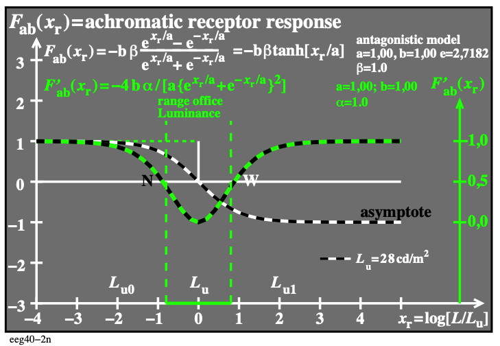
Fig. 4.47-4: Antagonistic receptor response (S-shaped) and its derivation (Gauss-shaped)
For the download of this figure in the VG-PDF format, see eeg40-2n.pdf.
For the achromatic receptor response and 2 antagonistic derivations, see Fig. 4.47-5.
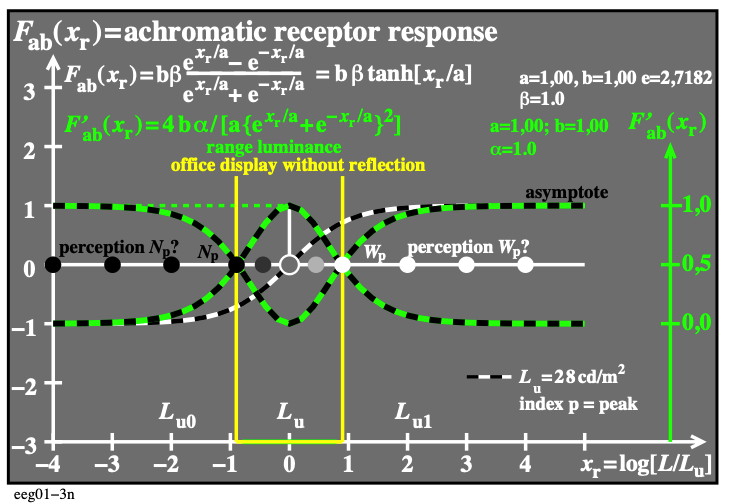
Fig. 4.47-5: Achromatic receptor response and 2 antagonistic derivations, perception of peak White & Black.
For the download of this figure in the VG-PDF format, see eeg01-3n.pdf.
On displays without reflection of the ambient light the contrast between White and Black may be C = 50:1.
For the achromatic receptor response and 2 antagonistic derivations, see Fig. 4.47-6.
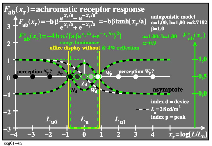
Fig. 4.47-6: Achromatic receptor response and 2 antagonistic derivations, luminance range of peak White & Black, and for contrast C = 90:3,6 = 25:1 (surface colour range).
For the download of this figure in the VG-PDF format, see eeg01-4n.pdf.
On displays with 3,6% reflection of the ambient light the contrast between White and Black may be C = 25:1. For mate surface colours this contrast is defined by the tristimulus values of White and Black YW : YB = 90 : 3,6.
For the achromatic receptor response and 2 antagonistic derivations, see Fig. 4.47-7.
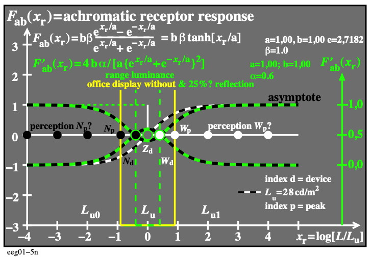
Fig. 4.47-7: Achromatic receptor response and 2 antagonistic derivations, luminance range of peak White & Black, and for contrast C=9:1 (25%? display reflection)
For the download of this figure in the VG-PDF format, see eeg01-5n.pdf.
On displays with 25% reflection of the ambient light the contrast between White and Black may be C = 9:1.
For the achromatic receptor response and 2 antagonistic derivations, see Fig. 4.47-8.
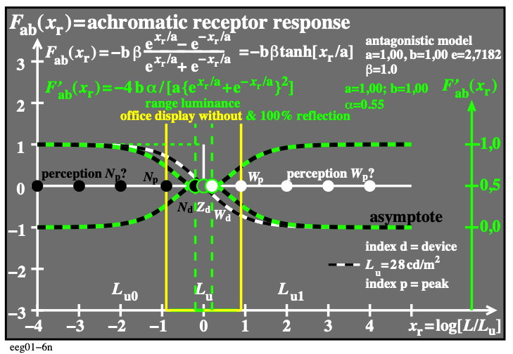
Fig. 4.47-8: Achromatic receptor response and 2 antagonistic derivations, luminance range of peak White & Black, and for contrast C=2:1 (100% display reflection)
For the download of this figure in the VG-PDF format, see eeg01-6n.pdf.
On displays with 100% reflection of the ambient light the contrast between White and Black is C = 2:1. In offices for surface colours the luminance is 5,6 cd/m^2 for black, 28 cd/m^2 for grey and 142 cd/m^2 for white. The luminance ratio is 25:1. If the luminance ratio is 2:1, then the white has a luminance by a factor 1,41 greater and the black a luminance by a factor 1,4 smaller compared to 28 cd/m^2. The perception of these two luminances is black and white, if the display is viewed. For example in this viewing situation the black text is produced by the lower luminance (20 cd/m^2) on the white screen of the higher luminance (39 cd/m^2).
4.48. Antagonistic response functions, summation, amplitude modulation, and derivation
The exponential response function can be splitted in two antagonistic functions, see Fig. 4.48-1.
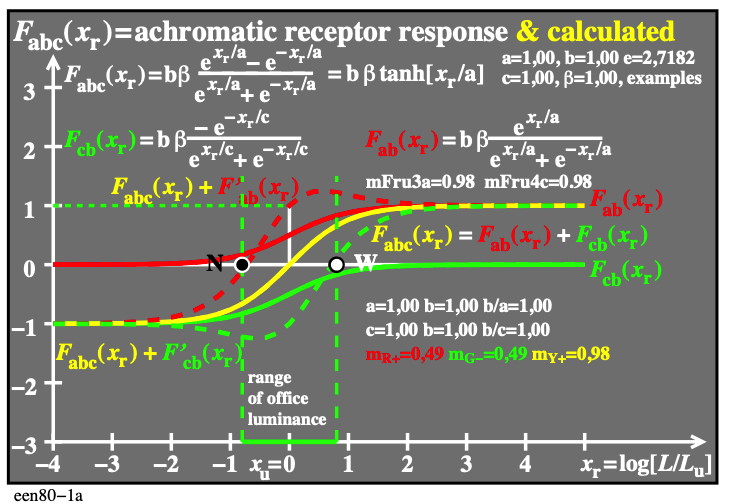
Fig. 4.48-1: Antagonistic response functions of equal slope, summation, and amplitude modulation
For the download of this figure in the VG-PDF format, see een80-1a.pdf.
The yellow function is the sum of both. A further sum or difference produce what is called amplitude modulation of electric signals. The antagonistic achromatic response and the chromatic reponse can be calculated from the signals of the amplitude modulation.
For the antagonistic response functions of equal slope, the summation, and the derivation, see Fig. 4.48-2.
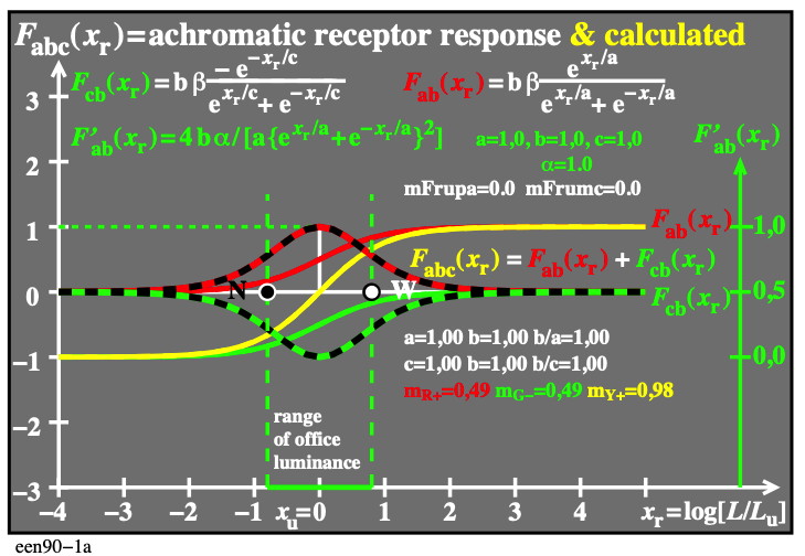
Fig. 4.48-2: Antagonistic response functions of equal slope, summation, and derivation
For the download of this figure in the VG-PDF format, see een90-1a.pdf.
For the antagonistic response functions of different slope, the summation, and the derivation, see Fig. 4.48-3.
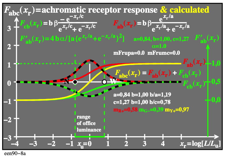
Fig. 4.48-3: Antagonistic response functions of different slope, summation, and derivation
For the download of this figure in the VG-PDF format, see een90-8a.pdf.
For the antagonistic response functions of equal slope, the summation, and the derivation of the response and the sum, see Fig. 4.48-4.
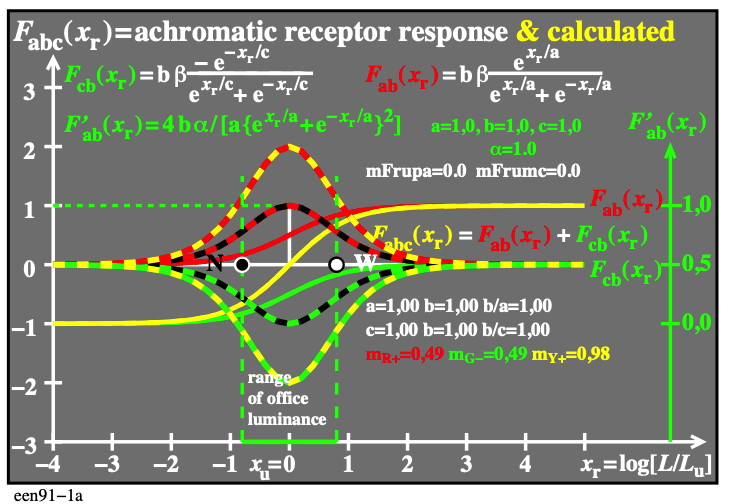
Fig. 4.48-4: Antagonistic response functions of equal slope, summation, derivation, and derivation of sum
For the download of this figure in the VG-PDF format, see een91-1a.pdf.
_________________________
For links to the main chapter E
Colour Metrics, Differences, and Appearance (2023), under work.
Content list of chapter E (links and file names use small letters), see
eea_s in English or ega_s in German.
This web page is since 2023 under work.
In future the figures and the text may be improved.
Link to the next topic (under work in 2023)
Title of part 4.5: Research results and connections of special CIE and TUB colourimetries
eea_s45 in English or ega_s45 in German.
-------
For the TUB start site (not archive), see
index.html in English, or
indexDE.html in German.
For the TUB archive site (2000-2009) of the BAM server
"www.ps.bam.de" (2000-2018)
about colour test charts, colorimetric calculations, standards,
and publications, see
indexAE.html in English,
indexAG.html in German.
For similar Information of the BAM server "www.ps.bam.de"
from the WBM server (WayBackMachine)
https://web.archive.org/web/20090402212108/http://www.ps.bam.de/index.html